Threat Research with Snowflake & VirusTotal

Lacework Labs·July 20, 2021·18 min read

There is no shortage of threat intelligence. Between numerous vendors and open sources, the amount of data can be overwhelming. The challenge then becomes curating what you already have and tailoring to your needs whether that’s for research, net defense, or both. Lacework Labs uses a number of different sources and tooling for this however we’ve derived the most value with a combination of Snowflake & VirusTotal; VirusTotal being the collection source, and Snowflake for data analysis and processing.

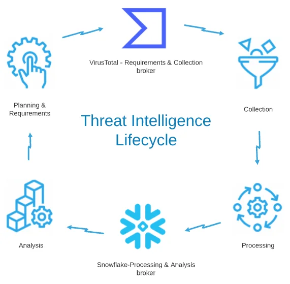
This blog is a how-to guide on collecting and analyzing threat intelligence with VirusTotal and Snowflake. We’ll describe how this applies to the phases of the intelligence life-cycle and include real-world examples showing how Lacework Labs is using Snowflake to extract indicators, and perform analysis tasks such as malware and attack-infrastructure clustering.

Only the key touchpoints of a collection process are covered in this blog. Details regarding deployment and scaling are out of scope.

Figure 1. Overview

Planning, Requirements Direction

The following are required for duplicating the tasks in this blog. (Collection requirements are listed in the following section.):

Snowflake datastore with read-write access role
VirusTotal API access
Python3 & Snowflake python connector
Lacework Labs tools and resources
- Collection & processing
- Analysis
  - AV clustering
  - Infrastructure clustering

Two Snowflake tables will be needed: “vt_collection_relations” (or your desired table name) for storing the VirusTotal API responses and timestamp data & “vt_clustering” for tracking of AV name clusters. These can be created with the following commands:

sha256 varchar(4096),
start_time timestamp_ltz(9),
end_time timestamp_ltz(9),
etl_time  timestamp_ltz(9),
PROPS variant);

create table vt_clustering (
sha256 varchar(4096),
cluster varchar(4096),
etl_time  timestamp_ltz(9),
PROPS variant);

Collection

Requirements will vary depending on use-case, however Lacework Labs currently collects information on malicious ELF binaries and bash malware. Hashes for files matching this criteria can be returned with the following queries:

Example Query	Description
tag:elf positives:1+ fs:2021-06-01+	Return hashes for files tagged as ‘elf’, with one or more AV detections and with a first_seen after June 1st 2021
tag:shell positives:1+ fs:2021-06-01+	Return hashes for files tagged as ‘shell’, with one or more AV detections and with a first_seen after June 1st 2021 ‘tag:elf positives:1+ fs:2021-06-01+’
name:*.sh positives:1+ fs:2021-06-01+	Return hashes for files with a .sh file extension, one or more AV detections and with a first_seen after June 1st 2021 .(Finds possible bash malware not tagged as shell files)

The next step in the Virus collection is to query the data for files that meet our requirements. One of these data-types is called relationships. VirusTotal provides valuable relational information regarding malware specimens such as IPs and domains seen as either artifacts or in the communication or distribution of the malware. The following are useful relationship types:

Relationship identifier	Description
itw_urls	Virus Total “In the Wild” URLs
itw_ips	IP addresses parsed from the ITW URLs
contacted_ips	IPs contacted during behavioral analysis
contacted_domains	Domains contacted during behavioral analysis
embedded_urls	Statically observable URLs

Using version 3 of the VirusTotal API, these relationship types can be returned with a single API request. Example implementation in Python:

def query_VT_behaviorv3(sha256):
        url = 'https://www.virustotal.com/api/v3/files/'+sha256+'?relationships=embedded_urls,itw_urls,itw_ips,contacted_ips,contacted_domains'
        proxies=None
        timeout=None
        response = requests.get(url,
                                headers={'x-apikey': api_key,
                                         'Accept': 'application/json'},
                                proxies=proxies,
                                timeout=timeout)
        if response.status_code != 200:
            print(response)
            raise
        return response.content

Processing

Snowflake can natively ingest JSON data (up to 16MB ) using the Variant universal data type. This reduces the need for parsing and simplifies both the processing and analytics of data returned from the VirusTotal API. The following is an insert example. Ingestion of the JSON data is achieved using the parse_json function.

1
2
3

INSERT into vt_collection_relations select column1 as SHA256,column2 as START_TIME,column3 as END_TIME,
 column4 as ETL_TIME, parse_json(column5) as PROPS from values ('80689dc14c3e0dda6a1786945679b10228893ea133573e011d4dda6acb6a038a', 
'2021-06-30 18:05:50', '2021-06-30 18:05:50', '2021-07-01 14:30:07', '{\n "data": "this is example json!"}');

Note – If using Python, it is important to write the raw Virus Total API response into Snowflake. If you convert to JSON using Python, then the resulting object will only be valid JSON for Python. For example, python renders null values as ‘None’. This may result in errors during Snowflake ingestion.

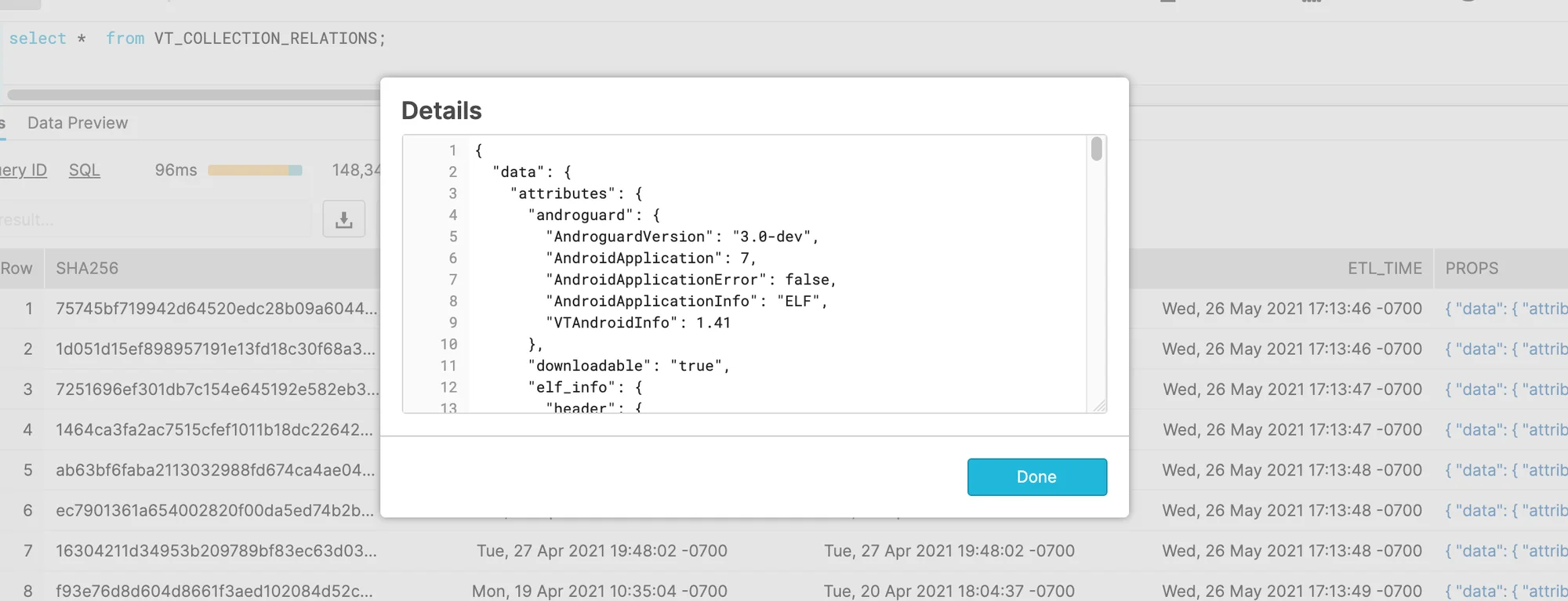Figure 2. VirusTotal JSON – Loaded into Snowflake

Analysis – Basic

The analysis phase of this collection lifecycle is where Snowflake stands out. This is due to its ability to query semi structured data within the Variant fields. For JSON data, this uses a special syntax to fetch the key-value pairs. The following is a simple example:

select distinct PROPS:data.attributes.tags from VT_COLLECTION_RELATIONS ;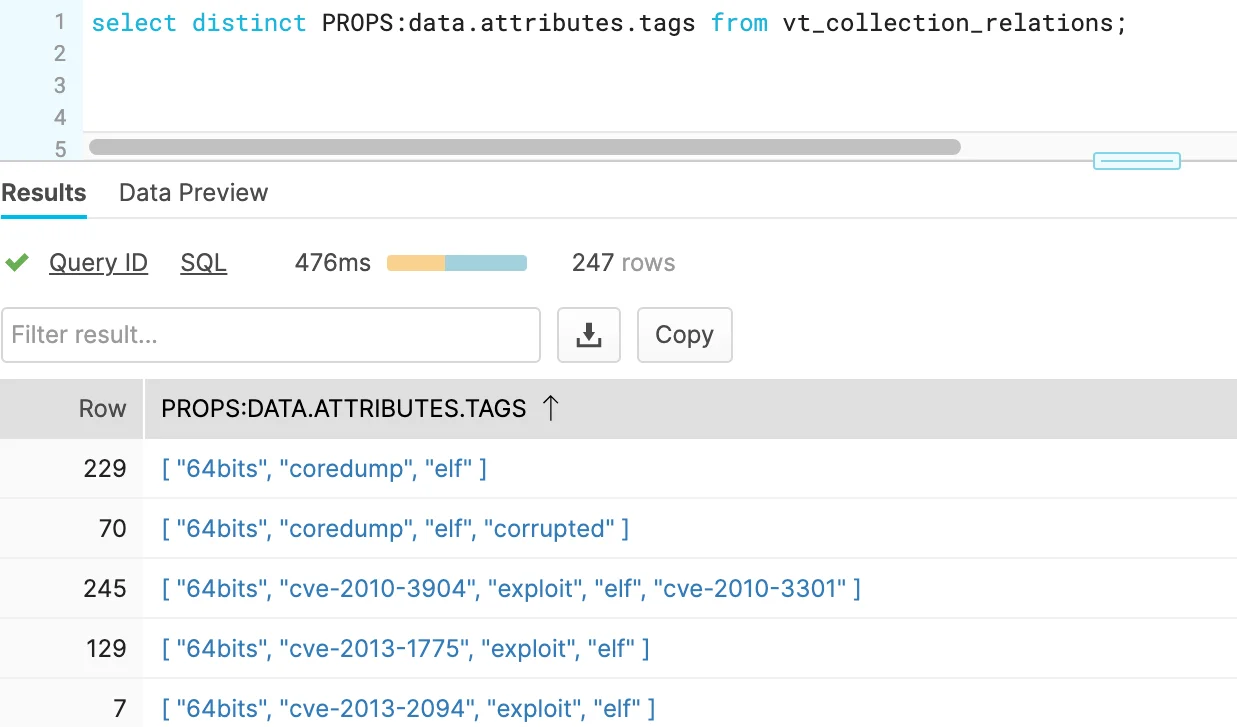

Figure 3. Parsed Tag Arrays

Figure 4 breaks down the components of this field query

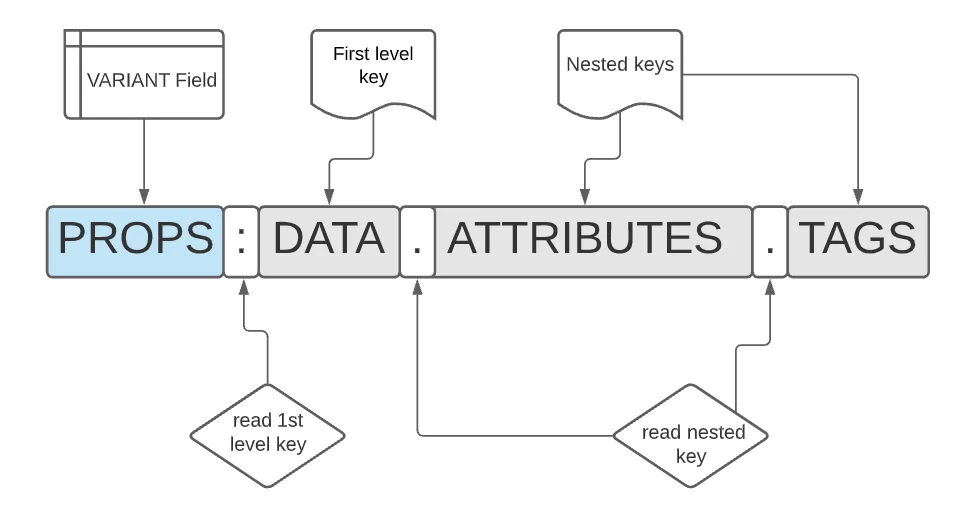Figure 4. Structured Query Breakdown

You’ll notice this query returns more structured data. If you’d like a single value per row, then the flatten function may be leveraged. Snowflake’s flatten function explodes values in an array into multiple rows for easier processing.

1
2

with vt as (select * from VT_COLLECTION_RELATIONS,
 lateral flatten(input => PROPS:data.attributes.tags) as value) select distinct(value) from vt;

This may further be refined – for example if we want to filter only tags pertaining to cves (common vulnerabilities and exposures). Example:

1
2
3

with vt as (select * from VT_COLLECTION_RELATIONS, lateral flatten(input => PROPS:data.attributes.tags)
 as value where PROPS:data.attributes.tags::varchar like '%cve%')
 select distinct(value) from vt where value like 'cve%' ;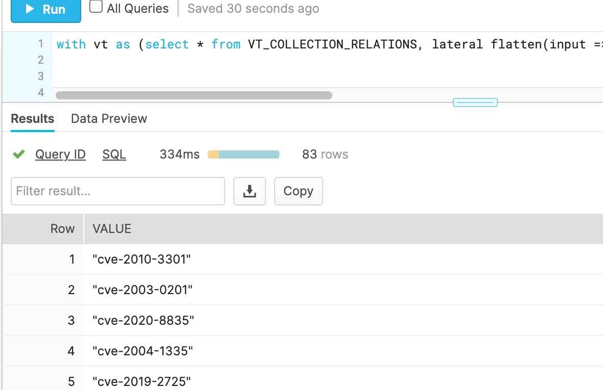

Figure 5. Flattened results

Ranking results can be achieved using counts and ‘order by’ modifiers. While these are not exclusive to Snowflake, they are especially useful in tandem with the structured data queries.

1
2

with vt as (select * from VT_COLLECTION_RELATIONS, lateral flatten(input => PROPS:data.attributes.tags) as value )
 select value, count(distinct SHA256) as fcount from vt where value like '%cve%' group by value order by fcount desc;

The PROPS:data.attributes.tags path is just one example. Similar queries may be performed for trending against all relationship types queried in the collection phase:

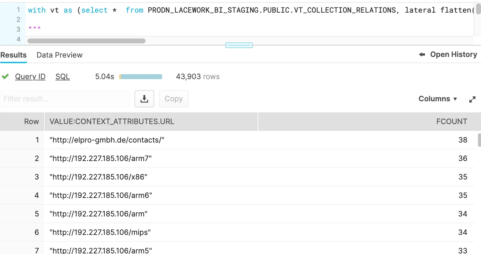Figure 6. Flattened results & counts

The following table shows possibilities when exploring this data set along with the flatten syntax:

Path	Description	Flatten example
PROPS:data.relationships.itw_urls.data	Virus Total “In the Wild’ URLs	with vt as (select * from VT_COLLECTION_RELATIONS, lateral flatten (input => PROPS:data.relationships.itw_urls.data) as value ) select value:context_attributes.url from vt;
PROPS:data.relationships.itw_ips.data	IP addresses parsed from the ITW URLs	with vt as (select * from VT_COLLECTION_RELATIONS, lateral flatten (input => PROPS:data.relationships.itw_ips.data) as value ) select value:id from vt ;
PROPS:data.relationships.contacted_ips.data	IPs contacted during behavioral analysis	with vt as (select * from VT_COLLECTION_RELATIONS, lateral flatten (input => PROPS:data.relationships.contacted_ips.data) as value ) select value:id from vt ;
PROPS:data.relationships.contacted_domains.data	Domains contacted during behavioral analysis	with vt as (select * from VT_COLLECTION_RELATIONS, lateral flatten (input => PROPS:data.relationships.contacted_domains.data) as value ) select value:id from vt ;
PROPS:data.relationships.embedded_urls.data	Statically observable URLs	with vt as (select * from VT_COLLECTION_RELATIONS, lateral flatten (input => PROPS:data.relationships.embedded _urls.data) as value ) select value:context_attributes.url from vt;
PROPS:data.attributes.last_analysis_results	Antivirus names	with vt as (select * from VT_COLLECTION_RELATIONS, lateral flatten (input => PROPS:data.attributes.last_analysis_results) as value ) select distinct value:result from vt ;

Analysis – AV Clustering

To successfully derive insights from any dataset, it is necessary to cluster items on common characteristics. In the bulk malware analysis category, clustering can be an ongoing challenge. This is especially relevant with VirusTotal as any given malware specimen can have over 50 different names from as many Antivirus scanners. Moreover, there can also be inconsistencies in AV names from a single vendor, not to mention 50+.

The value in VirusTotal however lies in name consensus. For example, if most AV vendors classify a specimen as “Mirai”, then this common substring may be used for clustering. The following are several examples showing multiple Mirai classifications for the same specimen.

ESET-NOD32 – A Variant Of Linux/Mirai.A
Fortinet – ELF/Mirai.B!tr
AegisLab – Trojan.Linux.Mirai.K!c
Rising – Backdoor.Mirai/Linux!1.CD3F (CLASSIC)
Zillya – Backdoor.Mirai.Linux.92696
Cyren – E32/Mirai.OT

The task then is to identify this common classification while also avoiding common generic substrings where possible (ie ‘backdoor’,’ELF’,’Linux’). While there would be many ways to achieve this, every method would need to involve substring parsing and ranking. But first, the AV names for our dataset will need to be extracted.

As mentioned in the previous section, AV names can be parsed with structured data queries within Snowflake. In this case however, we need both the AV name array and the SHA256 hash value which will be used for malware clustering. The following query fetches this data:

select sha256,PROPS:data.attributes.last_analysis_results from VT_COLLECTION_RELATIONS;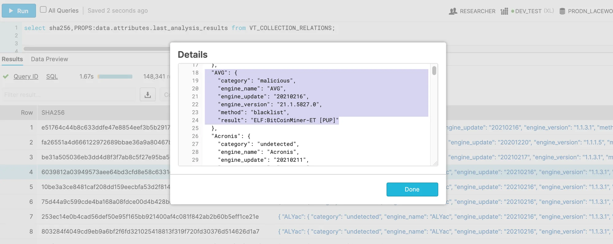

Figure 7. AV names query

Once we’ve returned the AV names from Snowflake, we can process with python. Since we’ve inserted raw JSON into Snowflake with the VARIANT data type, reading this data python simply involves a json.loadsI() call. Example

query = "select sha256,PROPS:data.attributes.last_analysis_results from VT_COLLECTION_RELATIONS;"

    cur.execute(query)
    for row in cur:
        sha256 = row[0]
        if sha256 in classified_files:
            already_processed += 1
            continue
        avnames =  json.loads(row[1])#load JSON from Snowflake!

Now we can start parsing common substrings to identify the consensus classification. As is the case in most programs, the answer can be found on Stack Overflow, in article – Using sequence matcher in Python to find the longest common string. This implementation allows for effective substring ranking.

The following is debug output using VirusTotal AV names as inputs. As you can see the common substrings are ranked by order of occurrence.

[160, 'mirai']
[57, 'linux']
[54, 'trojanlinuxmirai']
[25, 'ai']
[24, 'li']
[22, 'trojan']
[14, 'r']
…

From here, some post processing may be necessary to filter out the previously mentioned generic names and 2-3 character substrings. The result is a functioning malware classification system. These new cluster names can be written to vt_clusterstering table mentioned in Planning, Requirements Direction section.

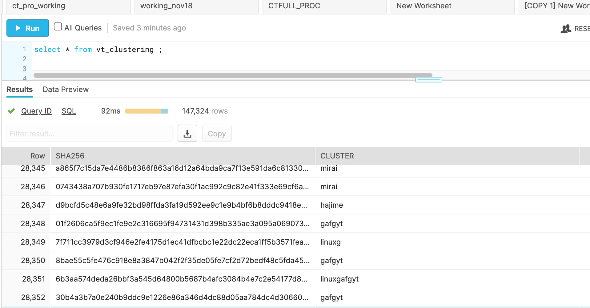Figure 8. AV names – clustered output

Saving clustered names in Snowflake will allow one to further refine classifications using the same process over common names across the data, as opposed to specific specimens. For example, generic classification ‘trojanlinux’ has many permutations that can only be seen after examining clustered names from multiple specimens.

- trojanlinuxagentbll
- trojanlinuxagentbmp
- trojanlinuxagentbnj
- trojanlinuxagentbop
- trojanlinuxagentbqs
- trojanlinuxagentbrw

Analysis – Infrastructure Clustering

Malware infrastructure clustering is simple relative to the AV name implementation. This is because fewer data points are involved. For example, AV clustering involves as many data points as there are AV names which in VirusTotal can be 50 or more. For network IOCs derived from VirusTotal, such as URLs, domains, and IPs this only involves domains, IPs, URLs, and URL components:

observed IPs and domains:
- static
- dynamic
observed URLs:
- full URL
- URL paths (URIs)
- URL file names (payloads)

Infrastructure component	Snowflake path(s)
Domains	PROPS:data.relationships.contacted_domains.data
IPs	PROPS:data.relationships.itw_ips.data PROPS:data.relationships.contacted_ips.data
URLs	PROPS:data.relationships.embedded_urls.data PROPS:data.relationships.itw_urls.data

With regards to ELF and bash malware, Lacework Labs has determined ITW_URLs (In the Wild) offer the most insights into malware distribution infrastructure. This is because a URL contains multiple pieces of information including, domains, IP address, URI paths, and payload file names. With Snowflake, these URLs can also be parsed using the using SPLIT and SPLIT_PART functions.

SPLIT Example – parsing and ranking hosts from URLs

1
2
3

with vt as (select * from VT_COLLECTION_RELATIONS, lateral flatten(input => PROPS:data.relationships.itw_urls.data)
 as value ) select SPLIT(value:context_attributes.url,'/')[2] as urlhost, count(distinct SHA256)
 as fcount from vt group by urlhost order by fcount desc;

SPLIT_PART Example– parsing and ranking payload names from URLs

1
2
3

with vt as (select * from VT_COLLECTION_RELATIONS, lateral flatten(input => PROPS:data.relationships.itw_urls.data) as value )
 select SPLIT_PART(value:context_attributes.url,'/',-1)
 as urlpayload, count(distinct SHA256) as fcount from vt where urlpayload not like '' group by urlpayload order by fcount desc;

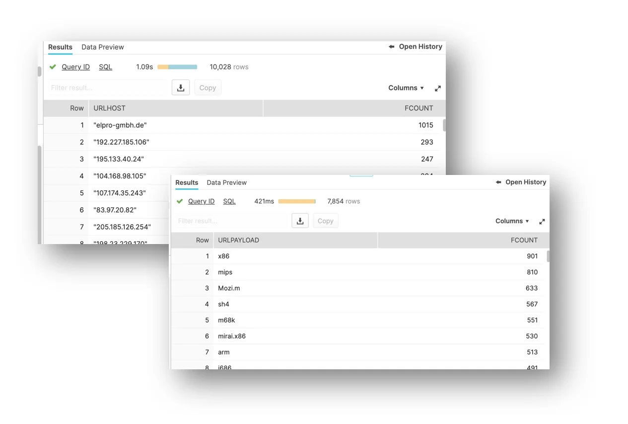Figure 9. Parsed URL component ranks – flatten +SPLIT + counts

With enrichment using the provided infrastructure clustering script, additional insights can be gleaned. The script generates an output that combines AV name clustering outputs along with URL component data.

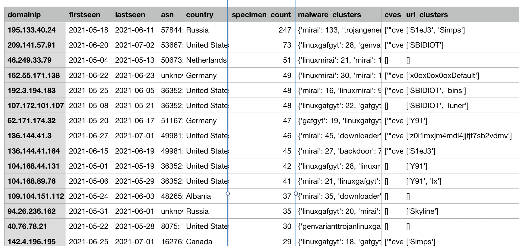Figure 10. Infrastructure clustering outputs

This URL link analysis is important as attackers often configure multiple infrastructures that can be either malware-specific, campaign specific, or both. One case study is Keksec, a prolific actor targeting cloud infrastructure. Keksec, uses various URI paths. For example:

http://23.95.8.110/Ryuk/ur0a.mips
http://45.14.224.197/Simps/i686
http://195.133.40.24/S1eJ3/IObeENwjarm6
http://107.172.156.158/Samael/i686

Using these URI paths as pivots, additional hosts can also be derived. Also, hosts that used two URIs can be used to link the components of this infrastructure. These were evident in the same infrastructure clustering outputs by sorting on the uri_clusters column. In the example below, the connections between the various portions of the Keksec infrastructure are apparent.

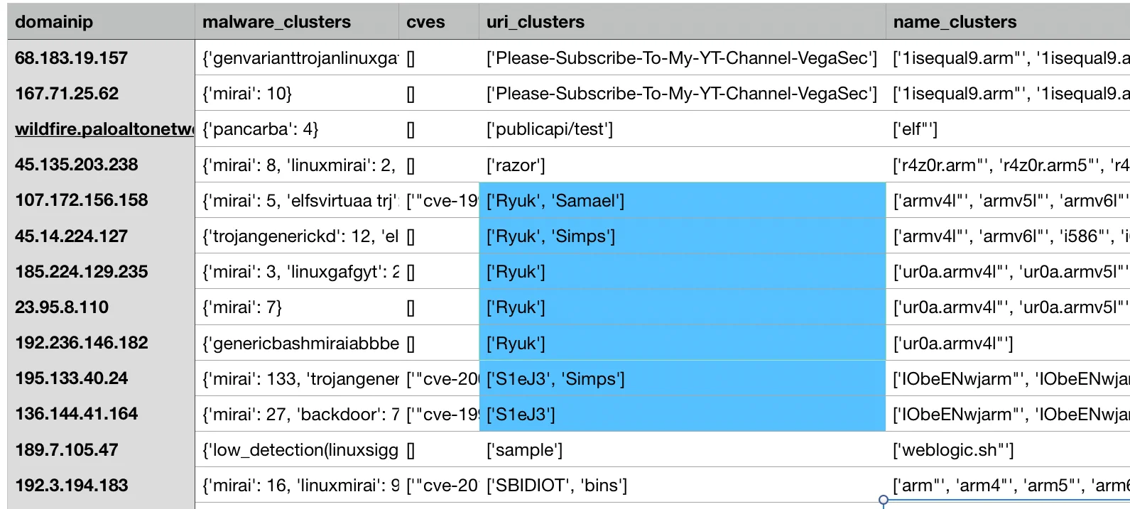Figure 11. Infrastructure clustering outputs – URI clusters

Payload pivoting can also help find infrastructure clusters and anomalies. For example, many Mirai campaigns leverage the same filenames so these can easily be grouped by sorting on this column. Alternatively, anomalous ITW hosts that are new and not observed as part of existing clusters may indicate emerging infrastructure and serve as early warning.

Conclusion

While 3rd party threat-intelligence providers offer value for many organizations, there is a lot to be said for curating your own from services like Virus Total. This involves more work however the result will be a higher detection efficacy as indicators can be tailored to your needs. One example from this blog would be the extraction of previously mentioned ITW URLs. These represent high fidelity indicators and have a low risk of false positive as they have already been observed distributing malware.

For those generating threat-intelligence from VirusTotal, additional tooling becomes necessary. Lacework believes Snowflake possesses a couple advantages in this regard: native processing of structured data & automated DBA tasks such as managed disk storage and compute sizing. This allows organizations to focus on the data instead of time-consuming administration and optimization tasks.

Tasks demo’d in this blog can be duplicated with the resources provided in Lacework Labs’ Github repository. If you found this blog useful then please share and follow us on LinkedIn and Twitter!